Differentiating Vector Fields on Manifolds

Affine Connections

Notion of derivative for vector fields on manifolds is called a connection , traditionally denoted by $\nabla$ ("nabla"). Given a tangent vector $u \in T_x\mathcal{M}$ and a vector field $V$, $\nabla_uV$ is the derivative of $V$ at $x$ along $u$. Formally, we should write $\nabla_{(x,u)} V$ where the base point $x$ is typically clear from context.
Note that we do not need a Riemannian metric yet.

Definition 1. A connection on a manifold $M$ is an operator

where:

• $\operatorname{T}_{}{\mathcal{M}}$ is the tangent vector space

• $\mathfrak{X}(\mathcal{M})$ denotes smooth vector fields on $\mathcal{M}$

This operator must satisfy four properties for all $u,w \in \operatorname{T}_{}{\mathcal{M}}$, $U,V,W \in \mathfrak{X}(\mathcal{M})$, $a,b \in \mathbb{R}$, and $f \in C^\infty(\mathcal{M})$:

1. Smoothness: $(\nabla_UV)(x) \stackrel{\Delta}{=}\nabla_{U(x)}V$ defines a smooth vector field $\nabla_UV$;

2. Linearity in $u$: $\nabla_{au + bw}V = a\nabla_uV + b\nabla_wV$;

3. Linearity in $V$: $\nabla_u(aV + bW) = a\nabla_uV + b\nabla_uW$;

4. Leibniz rule: $\nabla_u(fV) = \operatorname{D}{f}(x)[u]\cdot V(x) + f(x)\nabla_{u}{V}$.

The field $\nabla_U V$ is called the covariant derivative of $V$ along $U$ with respect to $\nabla$.

Theorem 2. Let $\mathcal{M}$ be an embedded submanifold of a Euclidean space $\mathcal{E}$. The operator $\nabla$ defined by

is a connection on $\mathcal{M}$, where $\operatorname{Proj}_{x}$ is the projector from $\mathcal{E}$ to the tangent vector space $\operatorname{T} _x(\mathcal{M})$.

Proof. Let $\mathcal{M}$ be an embedded submanifold of a Euclidean space $\mathcal{E}$ by $\bar \nabla$. Then

$$\nabla_u V = \operatorname{Proj}_{x} {\left(\operatorname{D}{\bar V}(x)[u]\right)} = \operatorname{Proj}_{x} {\left(\bar\nabla_{u}{\bar V}\right)}.$$

Projection is a linear operation which maintains the properties (linearities of $u, V$) of connections $\nabla_u V$, hence $\operatorname{Proj}_{x} {\left(\operatorname{D}{\bar V}(x)[u]\right)}$ is a connection on $\mathcal{M}$.

Proposition 3. Let $\mathcal{M}$ be a manifold with arbitrary connection $\nabla$. Given a smooth vector field $V \in \mathfrak{X}(\mathcal{M})$ and a point $x \in \mathcal{M}$, if $V(x) = 0$ then $\nabla_u V=\operatorname{D}{V}(x)[u]$ for all $u\in \operatorname{T}_{x}{\mathcal{M}}$. In particular, $\operatorname{D}{V}(x)[u]$ is tangent at $x$.

Riemannian Connections

Definition 4. For $U, V \in \mathfrak{X}(\mathcal{M})$ and $f \in \mathfrak{F}(\mathcal{U})$ with $\mathcal{U}$ open in $\mathcal{M}$, define:

• $Uf \in \mathfrak{F}(\mathcal{U})$ such that $(Uf)(x) = \operatorname{D} f(x)[U(x)]$;

• $[U, V]: \mathfrak{F}(\mathcal{U})\to \mathfrak{F}(\mathcal{U})$ such that $[U,V]f = U(Vf) - V(Uf)$;

• $\langle U, V\rangle \in \mathfrak{F}(\mathcal{M})$ such that $\langle U, V\rangle(x) = \langle U(x), V(x)\rangle _x$.

The notation $Uf$ captures the action of a smooth vector field $U$ on a smooth function $f$ through derivation, transforming $f$ into another smooth function. The commutator $[U,V]$ of such action is called the Lie bracket. Even in linear spaces $[U, V ]f$ is nonzero in general. Notice that $Uf = \langle \operatorname{grad}f, U\rangle$ owing to the definitions of $Uf, \langle V, U\rangle$ and $\operatorname{grad} f$.

Theorem 5. On a Riemannian manifold $\mathcal{M}$, there exists a unique connection $\nabla$ which satisfies two additional properties for all $U,V,W \in \mathfrak{X}(\mathcal{M})$:

1. Symmetry: $[U, V] f = (\nabla_{U}{V} -\nabla_{V}{U}) f$ for all $f \in \mathfrak{F}(\mathcal{M})$;

2. Compatibility with the metric: $U\langle V,W\rangle = \langle\nabla_{U}{V},W\rangle+\langle V,\nabla_{U}{W}\rangle$.

This connection is called the Levi-Civita or Riemannian connection.

Theorem 6. The Riemannian connection on a Euclidean space $\mathcal{E}$ with any Euclidean metric $\langle \cdot, \cdot \rangle$ is $\nabla_{u}{V} = \operatorname{D}{V}(x)[u]$: the canonical Euclidean connection.

Theorem 7. Let $\mathcal{M}$ be an embedded submanifold of a Euclidean space $\mathcal{E}$. The connection $\nabla_{}{}$ defined by Eq. 1 is symmetric on $\mathcal{M}$.

Theorem 8. Let $M$ be a Riemannian submanifold of a Euclidean space. The connection $\nabla_{}{}$ defined by Eq. 1 is the Riemannian connection on $\mathcal{M}$.

Proposition 9. Let $U,V$ be two smooth vector fields on a manifold $\mathcal{M}$. There exists a unique smooth vector field $W$ on $\mathcal{M}$ such that $[U,V]f = Wf$ for all $f \in \mathfrak{F}(\mathcal{M})$. Therefore, we identify $[U,V]$ with that smooth vector field. Explicitly, if $\nabla_{}{}$ is any symmetric connection, then $[U,V ] = \nabla_{U}{V} - \nabla_{V}{U}$.

Riemannian Hessians

Definition 10. Let $\mathcal{M}$ be a Riemannian manifold with its Riemannian con nection $\nabla_{}{}$. The Riemannian Hessian of $f\in \mathfrak{F}(\mathcal{M})$ at $x\in \mathcal{M}$ is the linear map $\operatorname{Hess} f(x): \operatorname{T} _{x}{\mathcal{M}} \to \operatorname{T} _{x}{\mathcal{M}}$ defined as follows:

Equivalently, $\operatorname{Hess}f$ maps $\mathfrak{X}(\mathcal{M})$ to $\mathfrak{X}(\mathcal{M})$ as $\operatorname{Hess}f[U] = \nabla_{U}{\operatorname{grad} f}$.

Proposition 11. The Riemannian Hessian is self-adjoint with respect to the Riemannian metric. That is, for all $x\in \mathcal{M}$ and $u, v\in \operatorname{T} _{x}{\mathcal{M}}$, $\langle \operatorname{Hess} f(x)[u], v\rangle _x = \langle u, \operatorname{Hess}f(x)[v]\rangle _x$.

Corollary 12. Let $\mathcal{M}$ be a Riemannian submanifold of a Euclidean space. Consider a smooth function $f : \mathcal{M}\to \mathbb{R}$. Let $\bar G$ be a smooth extension of $\operatorname{grad}f$— that is, $\bar G$ is any smooth vector field defined on a neighborhood of $\mathcal{M}$ in the embedding space such that $\bar G(x) = \operatorname{grad}f(x)$ for all $x \in \mathcal{M}$. Then, $\operatorname{Hess}f(x)[u] = \operatorname{Proj}_{x}{\left(\operatorname{D}\bar G(x)[u]\right)}$.

Connections as Pointwise Derivatives*

Definition 13. A connection on a manifold $\mathcal{M}$ is an operator

which has three properties for all $U ,V , W \in \mathfrak{X}(\mathcal{M})$, $f, g \in \mathfrak{F}(\mathcal{M})$ and $a, b \in \mathbb{R}$:

1. $\mathfrak{F}(\mathcal{M})$-linearity in $U$: $\nabla_{fU+gW}{V} = f\nabla_{U}{V} + g\nabla_{W}{V}$;

2. $\mathbb{R}$-linearity in $V$: $\nabla_{U}{(aV+bW)} = a\nabla_{U}{V} + b\nabla_{U}{W}$; and

3. Leibniz rule: $\nabla_{U}{(fV)} = (Uf)V + f \nabla_{U}{V}$.

The field $\nabla_{U}{V}$ is the covariant derivative of $V$ along $U$ with respect to $\nabla_{}{}$.

Proposition 14. For any connection $\nabla_{}{}$ and smooth vector fields $U,V$ on a manifold $\mathcal{M}$, the vector field $\nabla_{U}{V}$ at $x$ depends on $U$ only through $U(x)$.

Lemma 15. Given any real numbers $0 < r_1 < r_2$ and any point $x$ in a Euclidean space $\mathcal{E}$ with norm $\parallel \cdot \parallel$, there exists a smooth function $b: \mathcal{E}\to \mathbb{R}$ such that

• $b(y) = 1$ if $\parallel y - x \parallel \leq r_1$;

• $b(y) = 0$ if $\parallel y - x \parallel \geq r_2$; and

• $b(y) \in (0,1)$ if $\parallel y - x \parallel \in (r_1, r_2)$.

Using bump functions, we can show that $(\nabla_UV)(x)$ depends on $U$ and $V$ only through their values in a neighborhood around $x$. This is the object of the two following lemmas.

Lemma 16. Let $V_1, V_2$ be smooth vector fields on a manifold $M$ equipped with a connection $\nabla_{}{}$. If $V_1 \mid_\mathcal{U}= V_2 \mid_\mathcal{U}$ on some open set $\mathcal{U}$ of $\mathcal{M}$, then $(\nabla_{U}{V_1})\mid_\mathcal{U}= (\nabla_{U}{V_2})\mid_\mathcal{U}$ for all $U \in \mathfrak{X}(\mathcal{M})$.

Lemma 17. Let $U_1, U_2$ be smooth vector fields on a manifold $\mathcal{M}$ equipped with a connection $\nabla_{}{}$. If $U_1\mid_\mathcal{U}= U_2\mid_\mathcal{U}$ on some open set $\mathcal{U}$ of $\mathcal{M}$, then $(\nabla_{U_1}{V})\mid_\mathcal{U}= (\nabla_{U_2}{V})\mid_\mathcal{U}$ for all $V \in \mathfrak{X}(\mathcal{M})$.

Lemma 18. Let $U$ be a neighborhood of a point $x$ on a manifold $\mathcal{M}$. Given a smooth function $f\in \mathfrak{F}(\mathcal{U})$, there exists a smooth function $g\in \mathfrak{F}(\mathcal{M})$ and a neighborhood $\mathcal{U}^{\prime} \subseteq \mathcal{U}$ of $x$ such that $g\mid \mathcal{U}^{\prime} = f\mid\mathcal{U}^{\prime}$.

Lemma 19. Let $U$ be a neighborhood of a point $x$ on a manifold $\mathcal{M}$. Given a smooth vector field $U \in \mathfrak{X}(\mathcal{U})$, there exists a smooth vector field $V \in \mathfrak{X}(\mathcal{M})$ and a neighborhood $\mathcal{U}^{\prime} \subseteq \mathcal{U}$ of $x$ such that $V\mid_{\mathcal{U}^{\prime}} = U\mid_{\mathcal{U}^{\prime}}$.

Lemma 20. Let $U, V$ be two smooth vector fields on a manifold $\mathcal{M}$ equipped with a connection $\nabla$. Further let $\mathcal{U}$ be a neighborhood of $x \in \mathcal{M}$ such that $U| _{\mathcal{u}} = g_1W_1 + \cdots + g_n W_n$ for some $g_1, \dots, g_n \in \mathfrak{F}(\mathcal{U})$ and $W_1, \dots, W_n \in \mathfrak{X}(\upsilon)$. Then,

where each vector $(\nabla_{W_i}V)(x)$ is understood to mean $(\nabla_{\widetilde{W}_i}V)(x)$ with $\widetilde{W}_i$ any smooth extension of $W_i$ to $\mathcal{M}$ around $x$.

Differentiating Vector Fields on Curves

Induced Covariant Derivative

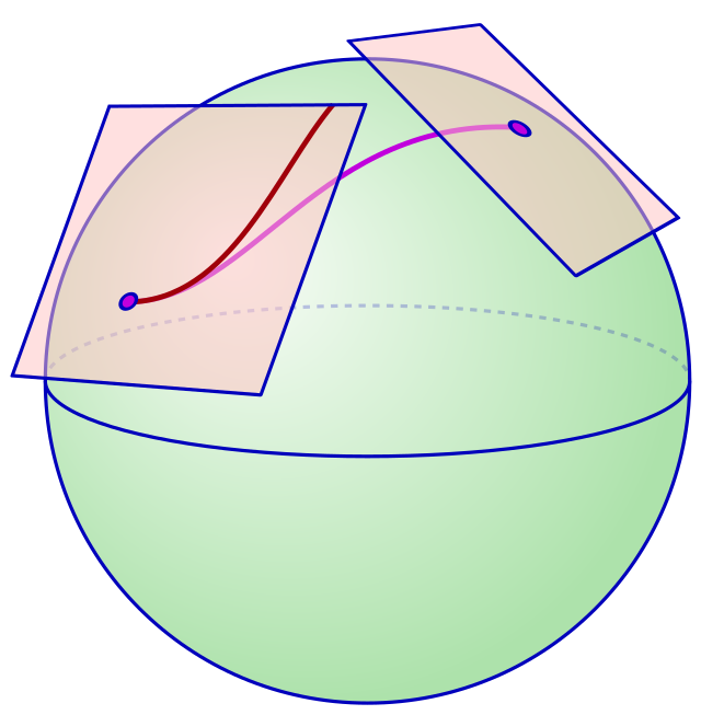
Definition 21. Let $c : I \to \mathcal{M}$ be a smooth curve on $\mathcal{M}$ defined on an open interval $I$. A map $Z : I \to \operatorname{T} _{}{\mathcal{M}}$ is a vector field on $c$ if $Z(t)$ is in $\operatorname{T} _{c(t)}{\mathcal{M}}$ for all $t \in I$. Moreover, $Z$ is a smooth vector field on $c$ if it is also smooth as a map from $I$ to $\operatorname{T} _{}{\mathcal{M}}$. The set of smooth vector fields on c is denoted by $X(c)$.

Theorem 22. Let $c \colon I \to M$ be a smooth curve on a manifold equipped with a connection $\nabla$. There exists a unique operator $\frac{D}{dt} \colon \mathfrak{X}(c) \to \mathfrak{X}(c)$ which satisfies the following properties for all $Y, Z \in \mathfrak{X}(c)$, $U \in \mathfrak{X}(\mathcal{M})$, $g \in \mathfrak{F}(I)$, and $a, b \in \mathbb{R}$:

1. $\mathbb{R}$-linearity: $\frac{D}{dt}(aY + bZ) = a\frac{D}{dt}Y + b\frac{D}{dt}Z$;

2. Leibniz rule: $\frac{D}{dt}(gZ) = \frac{dg}{dt}Z + g\frac{D}{dt}Z$;

3. Chain rule: $\left(\frac{D}{dt}(U \circ c)\right)(t) = \nabla_{c^{\prime}(t)}U$ for all $t \in I$;

4. Product rule: If $M$ is a Riemannian manifold and $\nabla$ is compatible with its metric (e.g., the Levi-Civita connection), then additionally: $$\frac{d}{dt}\langle Y, Z \rangle = \left\langle \frac{D}{dt}Y, Z \right\rangle + \left\langle Y, \frac{D}{dt}Z \right\rangle$$ where the inner product $\langle \cdot, \cdot \rangle$ along $c$ is defined by $\langle Y, Z \rangle(t) = \langle Y(t), Z(t) \rangle _{c(t)}$.

We call $\frac{D}{dt}$ the induced covariant derivative (induced by $\nabla$).

Proposition 23. Let $\mathcal{M}$ be an embedded submanifold of a Euclidean space $\mathcal{E}$ with connection $\nabla_{}{}$ as in Eq. 1. The operator $\frac{D}{dt}$ defined by $$\frac{D}{dt} Z(t) = \operatorname{Proj}_{c(t)}{\left(\frac{\text{d}{}}{\text{d}{t}} Z(t)\right)}$$ is the induced covariant derivative, that is, it satisfies properties 1–3 in Theorem 22. If $\mathcal{M}$ is a Riemannian submanifold of $\mathcal{E}$, then $\frac{D}{dt}$ also satisfies property 4 in that same theorem.

Acceleration and Geodesics

Definition 24. Let $c : I \to \mathcal{M}$ be a smooth curve. Its velocity is the vector field $c^{\prime} \in \mathfrak{X}(c)$. The acceleration of $c$ is the smooth vector field $c^{\prime\prime} \in \mathfrak{X}(c)$ defined by $c^{\prime\prime} = \frac{D}{dt} c^{\prime}$. We also call $c^{\prime\prime}$ the intrinsic acceleration of $c$.

When $\mathcal{M}$ is embedded in a linear space $\mathcal{E}$, a curve $c$ on $\mathcal{M}$ is also a curve in $\mathcal{E}$. It is then convenient to distinguish notationally between the acceleration of $c$ on the manifold (as defined above) and the classical acceleration of $c$ in the embedding space. We write

for the classical or extrinsic acceleration. In that spirit, we use notations $c^{\prime}$ and $\dot{c}$ interchangeably for velocity since the two notions coincide.

Definition 25. On a Riemannian manifold $\mathcal{M}$, a geodesic is a smooth curve $c : I \to \mathcal{M}$ such that $c^{\prime\prime}(t) = 0$ for all $t \in I$, where $I$ is an open interval of $\mathbb{R}$.

A Second-order Taylor Expansion on Curves

Lemma 26. Let $c(t)$ be a geodesic connecting $x = c(0)$ to $y = c(1)$, and assume $\operatorname{Hess}f(c(t)) \succeq \mu I$ for some $\mu\in \mathbb{R}$ and all $t\in [0,1]$. Then, $f(y) \ge f(x) + \langle \operatorname{grad}f(x), v\rangle _x + \frac{\mu}{2} \parallel v \parallel _x^2$.

Second-Order Retractions

Second-Order Retractions on Riemannian Manifold

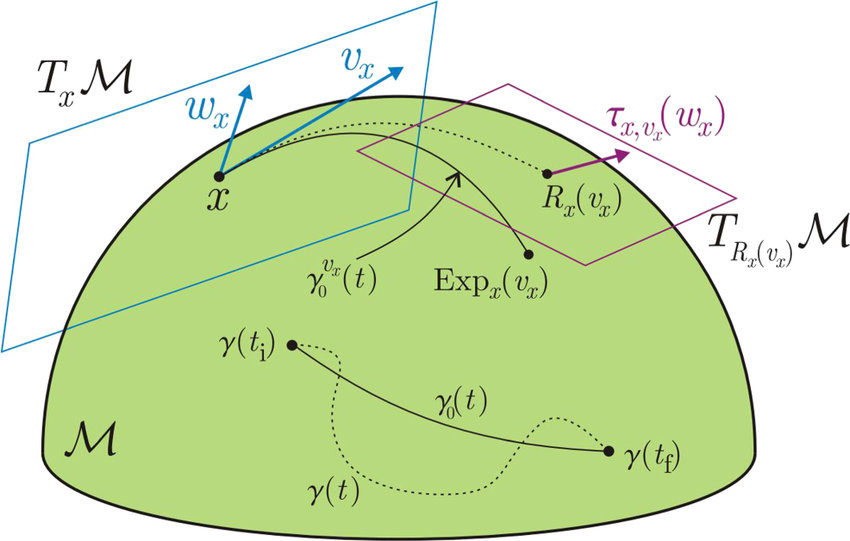
Definition 27. A second-order retraction $R$ on a Riemannian manifold $\mathcal{M}$ is a retraction such that, for all $x\in \mathcal{M}$ and all $v \in \operatorname{T}_{x}{\mathcal{M}}$, the curve $c(t) = R_x(tv)$ has zero acceleration at $t = 0$, that is, $c^{\prime\prime}(0) = 0$.

Proposition 28. Consider a Riemannian manifold $M$ equipped with any retraction $R$, and a smooth function $f: M \to \mathbb{R}$. If $x$ is a critical point of $f$ (that is, if $\mathrm{grad}f(x) = 0$), then

Also, if $R$ is a second-order retraction, then for all points $x \in M$ we have

Proposition 29. If the retraction is second order or if $\operatorname{grad} f(x) = 0$, then

where the right-hand side is the Hessian of $f \circ R_x : \operatorname{T} _{x}{\mathcal{M}} \to \mathbb{R}$ at $0 \in \operatorname{T} _{x}{\mathcal{M}}$. The latter is a “classical” Hessian since $\operatorname{T} _{x}{\mathcal{M}}$ is a Euclidean space.

Riemannian Submanifolds*

Metric Projection Retractions*